Copper Forward Curve: Why Spread Charts Miss the Mark
A single nearby spread tells you whether the copper forward curve is in contango or backwardation today. The full forward curve tells you where that structure changes, how steeply, and how long it persists. This information determines whether storing metal for three months profits more than storing it for twelve. That distinction is where delivery and storage decisions are made or lost.
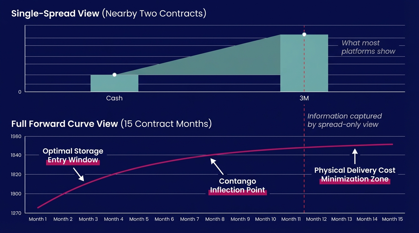
Relying exclusively on the cash-to-3-month spread produces a categorically different analysis from full-curve work. The single-spread view omits the structural information governing operational timing decisions. This post maps the specific decision points that become visible only when you build out the copper forward curve completely.
What Contango and Backwardation Mean in Copper Operations
Standard definitions establish the framework. Operational context determines how those definitions translate into tradeable decisions.
Contango in copper means the market is offering a premium for deferred delivery relative to prompt. In practice, this signals that holding physical metal (paying warehouse rent, insurance, and financing costs) can be offset or exceeded by the price differential between nearby and forward contracts. The curve is structurally offering compensation for storage.
Backwardation means the opposite: prompt copper commands a premium over deferred. The market is signaling that immediately available metal carries more value than future delivery. Financing and storage costs cannot be recovered by rolling forward. The curve is structurally penalizing storage.
Both structures carry direct operational consequences. Neither can be fully characterized by examining a single spread.
What Is Contango in Copper Futures Trading?
Contango in copper futures means the forward price exceeds the spot price after accounting for full carrying costs, including LME warehouse rent (approximately $0.47 per metric ton per day on LME-registered facilities LME fee schedule, financing at prevailing SOFR-linked rates, and insurance. When the price differential between, say, the 3-month and cash contracts exceeds total carry cost, the contango is "super-contango." This condition actively incentivizes warehousing metal rather than immediately delivering it.
The key operational distinction is that contango represents a profitability threshold with specific arithmetic rather than a mere directional signal. Whether that arithmetic closes in your favor depends on tenor. Tenor requires the full curve.
The Limits of a Single-Spread Chart in Copper Analysis
Most copper traders have two numbers on their screen: the cash price and the 3-month price. The spread between them is the first-line indicator of market structure. When cash trades below 3-month, the market is in contango. When cash trades above 3-month, backwardation.
That is serviceable shorthand until you need to make a decision that spans more than three months.
LME copper futures are listed with monthly expiries extending out to 63 months forward LME copper contract specifications. The cash-to-3-month spread covers roughly 2.4% of that total curve. Decisions made using only this spread are structurally incomplete regardless of how precisely the spread itself is tracked.
How Does a Full Forward Curve Differ From a Single Spread Chart?
A full forward curve maps the price of copper at every tradable maturity from cash out to five-plus years. A single spread chart shows only the relationship between two fixed points. The full curve reveals whether the contango or backwardation is uniform across all tenors, whether it reverses at a specific month, and how steeply the structure changes between delivery dates. A single spread can show direction; it cannot show shape, inflection, or persistence. Shape is where the actionable information resides.
Collapsing the curve to a scalar destroys the structure. This destruction systematically removes the inputs that physical operators need to make storage and delivery timing decisions with quantifiable confidence.
Reading the Full Copper Forward Curve: Three Decision Points
A properly annotated copper forward curve contains at least three distinct decision points that a single-spread view cannot surface. Each one maps directly to an operational decision with measurable P&L consequences.
Decision Point 1: The Carry Breakeven Tenor
The carry breakeven tenor is the forward maturity at which the cumulative contango premium exactly equals cumulative storage costs. Before that point, storage is unprofitable. After it, storage generates a positive spread.
For a trader holding physical copper and evaluating warehouse tenure, this is the minimum holding period that justifies warehousing versus prompt sale. On a single-spread chart, calculating this requires untestable assumptions about how the curve will evolve. On a full forward curve, it is visible directly: you locate the month where the price differential crosses your carrying cost threshold.
Published LME data shows total carrying costs for copper in a European LME-approved warehouse run approximately $8, 12 per metric ton per month depending on lot size and financing rate LME warehouse charges. A contango structure of $3/ton/month will not cover storage. A structure of $12/ton/month breaks even. The full curve shows you which months offer which structure. The nearby spread provides neither data point with structural precision.
Decision Point 2: The Curve Inflection Point
The inflection point is where the structure shifts, most commonly from steeper contango to flatter contango, or from backwardation to contango. Copper curves routinely exhibit mixed structures where the front end is in backwardation (reflecting near-term supply tightness) while the back end is in contango (reflecting long-run supply adequacy).
How Do You Read a Copper Forward Curve for Timing Decisions?
To read a copper forward curve for timing decisions, locate the inflection point where the slope changes direction or pace. If the front three months are in backwardation but months four through twelve flip to contango, that inflection date is your delivery timing signal: delivering before the inflection captures the backwardation premium; delivering after it requires absorbing contango cost. Identifying this point requires the full curve; it does not exist in the nearby spread.
In Q1 2024, LME copper exhibited exactly this structure: cash-to-3-month backwardation of approximately $50, 80 per metric ton while the 12-month calendar spread moved into mild contango LME copper historical data. A trader reading only the nearby spread would register "backwardation" and stop. A trader reading the full curve would identify the inflection around the four-to-five-month tenor and plan delivery timing accordingly. This is a structurally different and more precisely calibrated decision.
Decision Point 3: The Terminal Structure
The terminal structure is the long-end shape of the copper forward curve, indicating price behavior beyond 12 months. It does not affect short-term rolling decisions, but it governs medium-term physical procurement strategy, hedge ratios for annual offtake contracts, and capital allocation toward storage infrastructure.
A copper curve that is deeply backwardated at the front end but progressively steepens into contango in the back end signals a market expecting near-term tightness to resolve. The International Copper Study Group (ICSG) projects global copper mine supply to grow approximately 3.5% in 2025 while demand growth is forecast at 2.8%. This dynamic typically generates mild long-end contango while near-term inventory movements drive front-end volatility ICSG supply/demand forecasts. That structure (steeper backwardation near, flatter or inverted to contango far) is precisely the scenario where a single-spread read produces an incomplete picture of market positioning.
Storage Decisions the Full Copper Forward Curve Reveals
Physical storage decisions in copper are capital-intensive. LME-approved warehouses in Rotterdam, New Orleans, and Busan command significant per-lot costs. The decision to warehouse versus ship is strictly arithmetic, and that arithmetic requires the full curve.
When Should Copper Traders Use Forward Curve Analysis for Storage Decisions?
Copper traders should use full forward curve analysis for storage decisions whenever the holding period extends beyond one delivery cycle, which means consistently for physical operators. A single spread answers the question "should I store for three months?" The full curve answers "how long should I store, at which location, and when should I roll?" Those questions define the profitability of a storage position. Full curve analysis functions as the minimum analytical standard for physical operations.
The warehouse decision framework breaks into three executable steps:
- Map the carry breakeven tenor: identify the minimum holding period where contango covers your actual cost structure
- Identify the inflection point: determine whether holding beyond the breakeven tenor improves or degrades the spread
- Compare across delivery locations: LME premia vary by warehouse region; the spread that justifies storage in Detroit may not justify storage in Hamburg, and the full curve must be evaluated with location-specific cost inputs
LME Live data shows copper stocks in LME-registered warehouses have swung from under 100,000 metric tons to over 250,000 metric tons within 12-month windows multiple times in the past decade LME stock data. Those movements reflect exactly the kind of storage arbitrage decisions that become systematically visible on a full forward curve. They remain systematically obscured on a single-spread view.
Physical Delivery Timing and the Full Copper Forward Curve
Delivery timing decisions in copper carry direct P&L consequences. A mismatch between the delivery date contracted and the delivery date that maximizes spread can cost $20, 40 per metric ton on a prompt-to-nearby roll alone and compound significantly across a multi-month physical position.
What Does Backwardation Signal in Copper Physical Delivery?
Backwardation in copper physical delivery signals that the market is willing to pay a premium for immediately available metal, indicating localized supply tightness, warehouse stock drawdowns, or elevated short-term demand. For physical sellers, backwardation indicates a structural incentive to deliver promptly rather than defer. For physical buyers, backwardation is a cost signal: procuring today is structurally cheaper than procuring in 60 or 90 days, if the curve remains in that structure. The full curve is the only tool that quantifies whether that condition is likely to persist or resolve.
The operational risk backwardation creates in a single-spread workflow involves treating a tenored signal as a persistent one.
A front end backwardated by $80/ton on the cash-to-3-month spread might be backwardated by only $30/ton on the cash-to-6-month spread, and flat by month nine. A physical seller who reads "backwardation" from the nearby spread and delays delivery for six months expecting to capture the premium will find it largely eroded by the time they deliver. The full curve shows this directly; the nearby spread does not contain this information.
This matters significantly in copper because of per-unit value. Based on CME Group contract data, a single LME copper lot (25 metric tons) at $9,500/ton represents $237,500 in gross exposure CME/LME contract specifications. A $40/ton timing error across a 500-ton position is a $20,000 realized loss. Scaling that across annual physical volumes, full curve analysis functions as cost control as much as it does analytical enhancement.
Translating Copper Forward Curve Analysis Into Daily Workflow
Understanding the full copper forward curve analytically is one problem. Integrating it into daily trading workflow is a separate challenge. That second problem is where operational value is most frequently lost.
The practical bottleneck is data architecture. Most trading platforms surface the nearby spread as the default view because it is straightforward to display. Rendering the full forward curve (across 20-plus delivery months, updated in real time, with overlay analytics for carry thresholds and inflection detection) requires platform investment that most multi-commodity systems have not prioritized for copper specifically.
A 2023 Accenture survey on commodity trading operations found that approximately 67% of physical commodity traders reported relying on manual spreadsheet calculations for spread analysis outside their primary trading system Spreadsheet Comparisions. That figure reflects a platform gap rather than an analytical one. Traders understand the value of full curve visibility; their systems do not provide it without manual reconstruction.
Manual reconstruction introduces timing risk precisely when speed matters most. The workflow standard that copper forward curve analysis requires:
- Real-time full curve display: all tradable tenors, updated on live price feeds, not end-of-day snapshots
- Carry cost overlay: configurable financing rate and warehouse cost assumptions applied directly to curve shape so the breakeven tenor is computed, not estimated
- Inflection point detection: automated flagging of the tenor where curve slope changes direction, removing the need to identify it manually under time pressure
- Cross-venue spread comparison: simultaneous display of LME, COMEX, and SHFE copper curves, since location premia affect storage arithmetic independently of global structure
The Full Copper Forward Curve as Analytical Standard
The copper forward curve serves as an essential view. For any trader or physical operator making storage or delivery timing decisions, it is the primary analytical instrument. The nearby spread functions as a derived summary of it rather than the source.
The operational case is precise:
- Storage decisions made without the full curve cannot locate the carry breakeven tenor with structural precision
- Delivery timing decisions made without the inflection point are directionally oriented at best and structurally incomplete at worst
- Long-term procurement strategies built on the terminal structure require the back end of the curve, which the nearby spread does not contain
The single spread differs entirely from a condensed version of the full curve. It functions as a separate instrument that shares two data points with the curve while omitting the structural information that makes those points meaningful in context.
LME annual statistics rank copper among the most actively traded contracts on the exchange, with average daily volumes exceeding 400,000 lots across prompt dates LME annual statistics. The market liquidity to execute across the full curve already exists. The gap exists in the platforms rather than the market because building full-curve analytics for a single commodity requires genuine depth of focus that most platforms have not committed to.
Conclusion: The Curve Is the Position
The copper forward curve is the position. Everything else (the nearby spread, the front-month price, the real-time ticker) is a projection of it. Physical delivery and storage decisions are tenored decisions, and a single spread collapses tenure into a single number, discarding the structural information that makes those decisions tractable with precision.
Copper traders can immediately apply this analysis by taking three steps:
- Pull the full forward curve for your current position: map it out to at least 12 months, not just cash-to-3-month, and examine the actual shape, not just the sign
- Calculate your carry breakeven tenor: apply your actual financing rate and warehouse cost to identify where contango starts to cover storage in your specific cost structure
- Locate the inflection point: find where curve slope changes direction and build your delivery timing around that date, not around the nearby spread direction alone