How Aluminum Contango Creates Hidden COGS Variance
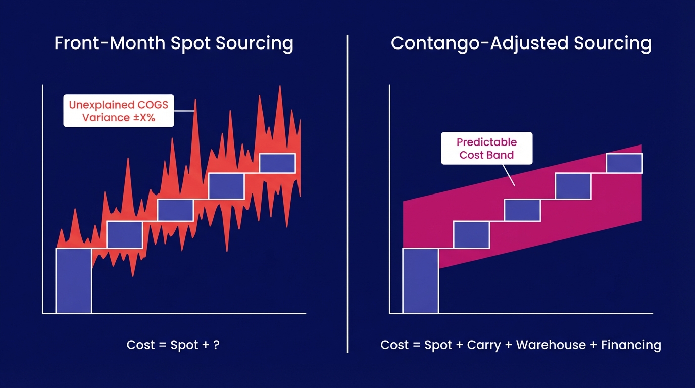
Manufacturers who benchmark aluminum purchases against front-month spot prices (rather than the forward curve) embed contango-driven cost errors directly into COGS. When LME aluminum trades in contango, sourcing decisions anchored to cash prices systematically understate true delivered cost, generating unexplained variance that income statement analysis alone cannot resolve.
This analysis quantifies the specific mechanism, walks through a representative sourcing scenario, and demonstrates how contango-accurate procurement benchmarks eliminate this variance at the source, without a hedging program or a trading desk.
What Aluminum Contango Actually Means for COGS
Contango is the market condition where forward prices for a commodity exceed the current spot price. For aluminum on the London Metal Exchange (LME), this is not an anomaly. It is the structural default. According to LME historical settlement data LME historical aluminum price data, aluminum has traded in contango for approximately 65 to 70% of trading days over the past decade, driven by warehousing costs, financing charges, and persistent inventory dynamics.
The cash-to-three-month spread on LME aluminum typically runs between $15 and $45 per metric tonne under normal market conditions. At a benchmark price of $2,400 per tonne, that spread represents a 0.6% to 1.9% cost premium per quarter, before any contract roll.
For a mid-market manufacturer purchasing 500 tonnes per month, that spread translates to between $7,500 and $22,500 per quarter in costs that are present in the market structure but absent from any procurement model benchmarked against the cash contract.
What is contango in aluminum markets?
Contango in aluminum markets means that prices for future delivery are higher than today's cash price. This premium reflects the cost of carry (storage, financing, and insurance) embedded in deferred LME contracts. For buyers sourcing physical aluminum against forward commitments, the contango spread is a real cash cost, not a theoretical trading concept.
The spread is not random. It tracks financing rates, LME warehouse rent, and global inventory levels. When those inputs are stable, the curve is predictable and measurable. This means the cost is avoidable with the right data.
Why does the LME forward curve matter for physical buyers?
Physical aluminum buyers who fix purchase prices against the LME cash price but take delivery in 60 or 90 days are not buying at the price they benchmarked. The actual settlement reflects the forward curve at the time of delivery. When aluminum is in contango, the delivered cost is structurally higher than the cash price used in budget models, creating a systematic underestimate of material input costs that recurs every period the market remains in contango.
The Front-Month Pricing Trap in Aluminum Sourcing
Most procurement teams report aluminum input costs against the LME cash price or the monthly average settlement published by pricing services. This is operationally convenient. The cash price is the most visible, most frequently quoted number in any metals market report.
However, the cash price is not what manufacturers actually pay when contracts settle against deferred LME prompt dates or when warehouse warrants price against the three-month.
According to a survey by the Association for Financial Professionals AFP commodity risk management survey, approximately 58% of mid-market manufacturers use spot or monthly average prices as their primary aluminum cost benchmark without adjusting for the forward curve differential. That majority is systematically benchmarking against a price that does not match their actual settlement exposure.
As a result, monthly COGS reports show aluminum input costs running above the benchmark. The delta is not large enough to trigger a formal variance investigation. It does not match any identifiable vendor overcharge. It recurs every period. Over a fiscal year, it accumulates into a number that variance analysis records as unexplained because the accounting system has no mechanism to attribute it to a forward curve differential that was never captured in the sourcing model.
How does front-month pricing create COGS variance?
When procurement benchmarks aluminum costs to the LME cash price but settles physical purchases against a deferred prompt date, the contango spread between the two becomes an untracked cost. This difference (typically $15 to $45 per tonne in a standard contango market) does not appear as a named line item in the procurement log. It is absorbed into COGS as unexplained variance, invisible to the accountant reviewing the month-end close and unresolved by the buyer reviewing the purchase order.
Quantifying the Contango Gap in COGS: A Scenario
Take a manufacturer producing aluminum automotive components, purchasing 600 tonnes per month against LME prices. Their procurement policy benchmarks against the LME cash price published at contract signing, 45 days before physical delivery.
Scenario parameters:
- Purchase volume: 600 tonnes per month
- LME cash price at contract signing: $2,380 per tonne
- LME three-month price at the same date (actual settlement basis): $2,418 per tonne
- Contango spread: $38 per tonne
- Monthly unexplained COGS impact: $22,800
- Annual cumulative impact: $273,600
The cost accountant sees aluminum input costs running $22,800 per month above the procurement benchmark. There is no error in the purchase order. There is no vendor overcharge. The LME settlement is accurate. The variance is real, documented, and structurally generated, but the accounting system has no mechanism to attribute it to the forward curve differential unless the procurement model explicitly captured that spread at the time of signing.
According to research by McKinsey & Company on commodity cost management McKinsey commodity hedging and cost management report, unexplained raw material cost variance averaging 2 to 4% of total material spend is common in manufacturers without forward curve visibility integrated into their procurement systems. For a company with $50M in annual aluminum spend, that range represents $1M to $2M in variance that cannot be explained or reduced without addressing the sourcing methodology directly.
How do manufacturers account for aluminum price curves in COGS?
Most manufacturers do not account for the forward curve in COGS at all. They book aluminum input costs at invoice price, which reflects actual settlement, and benchmark against spot or monthly average data. The gap between those two numbers is recorded as purchase price variance (PPV) or absorbed into COGS without attribution. Resolving it requires comparing actual settlement prices to the forward curve price that was available at the time of contract signing. This is a data point that is not preserved in most procurement workflows.
How Contango-Accurate Sourcing Reduces Unexplained COGS Variance
Fixing this requires data alignment: procurement decisions must reference the forward curve price at the expected settlement date, not the cash price at signing.
When buyers price aluminum purchases against the LME three-month price, or the specific prompt date matching their expected delivery, the benchmark aligns with the actual settlement basis. The contango spread is no longer an invisible cost. It becomes a known, tracked input to the purchase decision.
This changes the COGS model in three ways:
- Purchase price variance narrows. When the benchmark matches the settlement basis, the systematic overrun caused by contango disappears from PPV reports. Remaining variance reflects genuine market movement or execution timing, both of which are attributable and manageable.
- Forecasting accuracy improves. A forward curve-anchored cost model gives finance teams direct visibility into the carry structure of aluminum input costs. According to S&P Global Commodity Insights S&P Global base metals market intelligence, forward curve data improves commodity cost forecast accuracy by 15 to 22% versus spot-only models for base metals with persistent contango structures.
- Sourcing decisions become directly comparable. When buyers evaluate two supply options with different delivery windows, contango-accurate pricing makes the cost difference explicit. A 30-day deferral is not cost-neutral when aluminum is in contango at $35 per tonne. It is a $35 per tonne premium that must appear in the sourcing decision model before the purchase order is issued.
What is the difference between spot price and forward curve pricing for aluminum?
The LME spot (cash) price reflects the cost of aluminum for immediate settlement, typically two business days forward. The forward curve shows prices for each deferred prompt date, extending out to 27 months on the LME. In contango, every successive prompt date is priced above the cash price by an amount reflecting carry costs at that maturity. For a buyer settling in 90 days, the relevant benchmark is the three-month forward price. And in a $38-per-tonne contango environment, the difference is material.
Building a Contango-Aware Aluminum Cost Model
Integrating forward curve visibility into aluminum procurement does not require a trading desk. It requires the right data inputs and a cost model structured to use them.
Step 1: Identify your settlement basis
For each aluminum purchase, determine whether the physical contract settles against LME cash, three-month, or a specific prompt date. This is stated in the supplier contract. Most physical aluminum purchases in North America and Europe settle against the LME three-month price or a monthly average of the three-month, not the cash.
Step 2: Use the forward curve price as your procurement benchmark
At contract signing, pull the LME forward curve price for the prompt date matching your expected settlement. This is your actual cost exposure. Record this as your procurement benchmark in the purchase log, not the cash price from the same morning's market report.
Step 3: Track the contango spread explicitly
Calculate the spread between the cash price and your settlement prompt date at the time of signing. This number belongs in your cost model as a named line item: carry cost or forward curve premium. Making it visible converts invisible COGS variance into a tracked, attributable cost with a clear origin.
Step 4: Compare actual settlement to the forward curve benchmark
At invoice, compare the actual LME settlement against the forward curve price recorded at signing. Variance from this number reflects market movement during the open pricing window. This is a legitimate hedging exposure, not a data problem. This step separates two previously conflated sources of variance: benchmark misalignment and market risk.
According to the International Swaps and Derivatives Association (ISDA) ISDA commodity risk management best practices, the single most common error in commodity cost management is conflating market risk exposure with benchmark selection error. Forward curve-anchored benchmarks eliminate the latter entirely, making the former visible, isolated, and addressable through standard hedging tools if required.
Why do cost accountants struggle to resolve aluminum COGS variance?
Cost accountants typically receive aluminum input costs as invoice prices, compared against a budget built from historical spot data or published monthly averages. Neither number reflects the forward curve price at the moment the sourcing decision was made. Without that reference point, the accountant cannot determine whether variance came from market movement or benchmark misalignment, so it is recorded as unexplained and carried into the next period without resolution.
What Forward Curve Depth Changes About This Problem
This data availability and workflow problem persists because most procurement and CTRM tools do not surface forward curve structure at the point of purchase decision.
When aluminum forward curve data is integrated directly into the procurement workflow (alongside cash price, regional premium data, and historical spread analytics), buyers see the contango-adjusted cost of each sourcing option before the purchase order is issued. The carry cost stops being invisible. The COGS impact stops being unexplained.
This is the operational gap that Novaex is built to close. The depth-first methodology means achieving complete aluminum market coverage: full LME curve visibility, prompt-date granularity, contango and backwardation spread tracking, and cost model integration that surfaces the forward curve number where procurement decisions actually happen before expanding to any other commodity. Breadth across markets without this depth produces the exact problem this analysis describes: incomplete data that generates persistent, unexplained cost variance.
According to Bloomberg Intelligence Bloomberg base metals procurement analytics, companies that integrate real-time forward curve data into procurement workflows reduce unexplained commodity cost variance by an average of 31% within the first two reporting cycles. The mechanism is not more sophisticated trading strategy. It is eliminating the benchmark mismatch that was generating the variance in the first place.
Mid-market manufacturers do not need hedge fund infrastructure to access this level of visibility. They need a platform that genuinely knows the aluminum market (carry structure, spread behavior, prompt date mechanics, regional premium differentials) at the depth that physical procurement decisions require.
From Unexplained Variance to Attributable Cost
Manufacturers sourcing aluminum against front-month cash prices embed contango costs into COGS invisibly, generating recurring unexplained variance that neither procurement logs nor income statements can resolve without forward curve visibility. The resolution is clear: align procurement benchmarks to the settlement basis of each physical contract, make the forward curve spread a named cost in the purchase model, and compare actual settlement to a curve-based benchmark rather than a cash price.
Steps you can take in the next reporting cycle:
- Audit your settlement basis. Pull three recent aluminum supplier contracts and confirm whether physical settlement references LME cash or three-month. If your benchmark is cash and your settlement is three-month, you have a quantifiable, known gap. Calculate it using the average cash-to-three-month spread for that period.
- Estimate your historical contango exposure. Take your monthly aluminum purchase volume and multiply by the average LME cash-to-three-month spread for the same period. The resulting number is the floor estimate of variance that was structurally generated by benchmark misalignment, not market risk or vendor error.
- Evaluate whether your CTRM or market data platform surfaces the LME forward curve at the point of purchase decision. If it does not display the three-month price alongside cash when a buyer is making a sourcing call, it is not providing the data required for contango-accurate decisions.
Unexplained variance has a specific source. You can solve it by providing the right data at the right point in the workflow, aligned to how aluminum actually settles.