How Exchange Tick Data Degrades in the Metals Pipeline
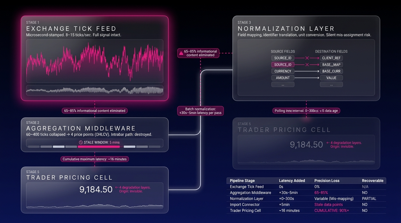
Physical metals pricing breaks originate at the exchange tick feed, not the trader's spreadsheet. By the time LME or COMEX data reaches a position management system, it has passed through four distinct degradation stages, each discarding a measurable portion of the precision the original signal contained. The break is structural and pre-trader.
This article identifies each pipeline stage, quantifies the degradation it introduces, and establishes why the pricing error traders encounter in their systems was determined before any human made a decision.
The Five Stages of Physical Metals Pricing Data Degradation
The data pipeline between an exchange matching engine and a metals trader's pricing cell is not a single pipe. It is a chain of five sequential processing stages, each with its own failure mode.
The stages, in order, are:
- Exchange tick feed: microsecond-stamped raw trade and quote events
- Aggregation middleware: tick compression into time-interval bars
- Normalization layer: field mapping, identifier translation, and unit conversion
- Import connector: the bridge between market data infrastructure and the CTRM/ETRM platform
- Spreadsheet cell: the downstream display layer where traders first encounter the degraded signal
The contents of exchange tick data
Exchange tick data is the raw, event-level output of a matching engine. Each tick record contains a timestamp (typically microsecond precision on modern venues), instrument identifier, price, quantity, and trade type. During LME Ring session and electronic trading hours combined, front-month copper (LME Grade A) produces between 12,000 and 45,000 individual tick events per trading day depending on volatility. This is the uncompressed signal at full precision.
The subsequent aggregation stage permanently replaces this resolution.
Stage 1: Exchange Tick Feed (The Uncompressed Signal)
The exchange tick feed is the only point in the pipeline where the full price signal exists in its original form. Every trade and quote change is preserved with microsecond-level timestamps and exact lot sizes.
According to CME Group's market data documentation, the Globex matching engine timestamps events at nanosecond resolution internally, with feed-level precision at microseconds. LMEselect and SHFE electronic platforms operate at comparable tick resolution for their listed base metals contracts.
This precision is operationally significant for physical metals because basis relationships, the spread between exchange futures and physical spot, can shift by $3, $8 per tonne within seconds during active LME Ring sessions. A risk system consuming tick-level data has the raw material to compute real-time basis with full intraday resolution. A system consuming aggregated bars does not. LME Ring session pricing mechanics
During peak Ring session activity, LME front-month copper generates approximately 8, 15 tick events per second on a normal trading day, with bursts exceeding 40 ticks per second during high-volatility events. Over a full session, this produces a complete, granular record of every price formation event. This dataset is irreversibly compressed in the next stage.
Stage 2: Aggregation Middleware (Where Physical Metals Pricing Data Precision Collapses)
Aggregation middleware sits between the raw exchange feed and every downstream consumer. Its function is to reduce tick data volume into a manageable format, typically Open-High-Low-Close-Volume (OHLCV) bars at fixed time intervals: 1-second, 1-minute, or 5-minute.
The compression ratio is significant and non-recoverable. A 1-minute OHLCV bar for LME copper during an active session collapses between 60 and 400 individual tick events into four price points and one volume figure. A 5-minute bar collapses between 300 and 2,000 ticks into the same five fields.
The precision losses at this stage operate across three dimensions:
- Timestamp degradation: Microsecond tick timestamps are replaced by the bar's closing timestamp. All intrabar price formation is invisible to downstream systems.
- Intrabar price extreme erasure: According to a 2022 analysis by the CFA Institute on market microstructure data quality, time-bar aggregation eliminates between 65% and 85% of the informational content present in raw tick data for actively traded commodity futures. CFA Institute market microstructure report The actual traded high and low within a minute are frequently not identical to the bar's H and L values when liquidity is thin or when a large order sweeps multiple price levels within the interval.
- Volume attribution loss: When trades are aggregated into bars, the relationship between individual lot sizes and price levels is permanently destroyed. A 500-lot trade at $9,200/tonne and a 10-lot trade at $9,215/tonne appear only as aggregate volume in the bar. The size-price relationship required for accurate VWAP or weighted average price calculation is eliminated.
Tick data vs. OHLCV bar data in metals pricing
Tick data is a complete, event-level record of every price change and trade, preserving the exact sequence, size, and timestamp of each price movement. OHLCV bar data is a four-point summary of activity within a fixed time window, with all intrabar detail permanently discarded. For physical metals pricing, this distinction is operationally critical: tick data preserves the intrabar price path required to accurately mark physical positions against prompt dates, while OHLCV bars cannot reconstruct what happened within the aggregation window, making them structurally inadequate for precise basis calculation during volatile sessions.
Most commodity trading operations accept this compression as a necessary cost of data volume management. The cost is real and measurable: the aggregated bar is not a complete representation of market activity within that interval. It is a four-point summary that permanently discards the majority of the price formation events that occurred.
Stage 3: Normalization Layer (Where Meaning Gets Reassigned)
The normalization layer transforms aggregated bar data from the exchange's native format into a standardized schema compatible with the downstream CTRM or ETRM platform. This stage performs three operations, each introducing its own error class.
Field mapping translates exchange-native field names and data types into the platform's internal schema. A mapping error (for example, routing LME cash settlement price to a field intended for the three-month futures price) produces a pricing error that is structurally invisible to the system. No validation check flags a numerically plausible price assigned to the wrong contract type. The error surfaces only when a trader or reconciliation process compares the position price against an external reference.
Instrument identifier translation converts exchange-native instrument codes to internal identifiers. When translation tables are not updated after an exchange metadata change (a contract expiry roll, a new prompt date, or a code revision), the normalization layer silently assigns incoming prices to the wrong instrument. LME instrument code structures are updated on a quarterly schedule; organizations that do not maintain synchronized identifier maps introduce systematic mis-mapping errors four times per year. LME contract specification management
Unit conversion transforms exchange-native units (LME prices in USD per tonne, COMEX prices in USD per pound) into platform-standard units. A conversion factor applied to the wrong field, or applied twice due to a pipeline configuration error, produces price errors that scale linearly with position size. A $0.01/lb conversion error on a 500-tonne copper position equates to an $11,023 mark-to-market discrepancy. This figure is large enough to affect hedging decisions but small enough to escape casual review.
How normalization introduces pricing errors
Normalization introduces pricing errors through three mechanisms: field mapping misassignment, instrument identifier translation failures, and unit conversion errors. Each mechanism can operate silently because the normalization layer has no semantic understanding of the contracts it processes; it executes transformation rules, but it does not validate that output prices are commercially coherent. Normalization latency in standard middleware implementations adds 20, 80ms per processing pass, and in batch-oriented architectures, the full normalization cycle runs at a configured interval rather than continuously, introducing an additional fixed delay of 30 seconds to 5 minutes.
Stage 4: Import Connector (Polling Gaps and the Stale Price Problem)
The import connector is the interface between the market data infrastructure and the CTRM or ETRM platform where physical positions are managed. In most legacy architectures, this connector operates on a polling model: it requests data from the upstream source at a fixed interval rather than receiving data as events occur.
Standard polling intervals in commodity trading platform implementations range from 1 minute to 15 minutes. A 5-minute polling interval (the most common default in mid-market CTRM deployments) means that position pricing can reflect data that is up to 300 seconds stale at any given moment.
CTRM import connector polling frequency
Most legacy CTRM import connectors are configured to poll market data sources at intervals between 1 and 15 minutes, with 5 minutes being the most common default configuration. This intended operating mode stems from batch-oriented import architectures designed when real-time data infrastructure was cost-prohibitive for mid-market operations. The polling interval defines the maximum possible data age; the average data age under a 5-minute polling cycle is approximately 2.5 minutes.
The stale price exposure this creates is directly quantifiable. During LME Ring session hours, copper prices routinely move $10, $25 per tonne within a 5-minute window on normal trading days. During high-volatility events (an unexpected macro data release, an LME inventory report, or a major producer announcement), 5-minute moves of $40, $60 per tonne are documented in LME historical data. LME historical volatility data
A 1,000-tonne copper position managed against data that is 300 seconds old during a $50/tonne move carries a mark-to-market error of $50,000, before any trader has made a single decision.
The import connector also introduces a second failure mode: connection state management. When an upstream data source is temporarily unavailable due to a feed interruption or maintenance window, the connector's behavior on reconnection determines whether the pricing gap is flagged or silently closed. In most default configurations, reconnection triggers a backfill that overwrites the last-known-good timestamp, and the system resumes as though no gap occurred. The stale interval is invisible in the audit log.
Stage 5: The Spreadsheet Cell (Where Breaks Become Visible)
By the time price data reaches a spreadsheet cell in a trader's workbook, it has passed through every degradation stage described above. The cell displays a number. It does not display the timestamp of the original tick, the aggregation interval that produced the bar, the normalization rules applied, or the polling lag of the import connector.
The trader sees a price. The price appears correct because it is a legitimately formatted, numerically plausible figure that passed every structural validation check in the pipeline. The discrepancy is entirely semantic.
The source of spreadsheet pricing discrepancies
Metals traders see pricing discrepancies in spreadsheets because the spreadsheet displays the output of a four-stage degradation pipeline, not the exchange price. The figure in the cell is accurate to the last import cycle, the last normalization pass, the last aggregation bar, and the last tick the aggregation middleware captured: four layers of compounding delay and precision loss, none of which are visible in the cell itself. Reconciliation against broker confirms or exchange settlement notices reveals the gap; the spreadsheet has no mechanism to surface it.
Spreadsheet-based systems add a fifth latency layer: refresh cycles. Workbooks connected to CTRM exports via ODBC or CSV refresh at intervals ranging from 15 seconds for live-linked sheets with efficient query optimization to 5 minutes for scheduled export-based workflows. According to a 2021 survey of commodity trading operations by Accenture, 67% of mid-market physical metals trading desks still use spreadsheet-based workflows for at least one critical pricing or risk function. commodity trading operations digitization survey
The cumulative end-to-end latency from exchange tick to spreadsheet cell in a typical legacy pipeline is:
| Pipeline Stage | Maximum Latency Added |
|---|---|
| Aggregation middleware (1-min bar) | 0, 60 seconds |
| Normalization layer (batch mode) | 30, 300 seconds |
| Import connector (5-min polling) | 0, 300 seconds |
| Spreadsheet refresh cycle | 15, 300 seconds |
| Total cumulative maximum | ~16 minutes |
When a trader prices a physical copper deal against a cell reflecting data from 16 minutes prior, the infrastructure has already introduced the pricing error. The trader is simply executing against its output.
Why Physical Metals Pricing Data Degradation Is Structural, Not a Configuration Problem
The degradation described above stems directly from the designed behavior of a pipeline architecture optimized for data volume management and infrastructure cost, rather than the precision requirements of physical metals pricing.
Aggregation exists because tick data volumes exceed the write throughput of conventional relational databases used in legacy CTRM platforms. A full tick capture for LME copper generates approximately 2, 4 gigabytes of raw data per trading day. Over a full year, that is 500GB, 1TB for a single instrument. This is a data volume that legacy platforms were not designed to query in real time. CTRM real-time data architecture options
Batch normalization exists because transformation operations are computationally expensive when applied event-by-event. Batching amortizes the cost across intervals at the price of latency. Polling connectors exist because push-based real-time interfaces require persistent connections and stateful error handling: an engineering complexity that legacy platforms deferred.
The cumulative result is a pipeline where physical metals pricing data degrades at every stage by design, and where the degradation is invisible to the system's users until a reconciliation failure, a missed hedge, or a disputed physical settlement surfaces the discrepancy.
According to a 2023 Gartner analysis of commodity management technology, organizations that rely on batch-oriented data pipelines for physical position management experience mark-to-market reconciliation breaks on 12, 18% of settlement cycles, with an average resolution time of 4.2 hours per break. The root cause in over 70% of cases traces to data pipeline latency rather than trader input error. The diagnosis belongs in the infrastructure rather than the front office.
Resolving structural physical metals pricing data degradation requires an architecture that eliminates aggregation as the default processing mode, runs normalization continuously rather than in batch cycles, and replaces polling connectors with event-driven data delivery. For base metals specifically (where basis, prompt date structure, and LME warehouse inventory interact in ways that are sensitive to intraday price formation), tick-level precision is not a premium feature. It is the minimum architectural standard for accurate position management.
How to Measure Your Pipeline's Degradation Profile
Understanding that degradation exists is the diagnostic starting point. Quantifying it for your specific pipeline requires measuring each stage directly rather than estimating from configuration parameters.
Four measurements produce a complete degradation profile:
- Aggregation interval audit: Identify the bar interval your aggregation middleware produces. Calculate the maximum intrabar precision loss for your primary instruments during representative volatility periods using documented LME or COMEX intraday price range data.
- Normalization batch interval: Determine whether your normalization layer runs continuously or in batch mode, and record the configured batch interval. Confirm whether the batch interval is enforced uniformly or varies under load.
- Import connector polling interval: Extract the polling configuration from your CTRM import connector for each market data source. Calculate worst-case staleness by multiplying the polling interval by your instruments' documented 5-minute realized volatility.
- End-to-end latency test: Record the timestamp of a known market event at the exchange level and trace it through each pipeline stage to its appearance in the trader-facing display layer. The elapsed time is your actual end-to-end latency, rather than an estimated configuration value. commodity data pipeline audit methodology
The Break Happens Before the Trader Arrives
Physical metals pricing breaks represent the predictable output of a four-stage data pipeline (aggregation middleware, normalization layer, import connector, spreadsheet refresh). Each stage operates as designed and discards a portion of the precision the exchange tick feed originally delivered. The exchange captures the price with full precision. Each successive pipeline stage systematically reduces that precision by design.
For physical metals trading operations where basis relationships, prompt date exposures, and real-time position visibility directly determine hedge execution quality, pipeline-introduced pricing errors are not a background operational nuisance. They are a quantifiable risk that surfaces in reconciliation breaks, disputed settlements, and hedges executed against prices that no longer reflect market reality.
Three immediate actions for metals trading operations:
- Run the four-step pipeline audit. Measure your actual end-to-end latency with a documented market event, not an estimated configuration value.
- Quantify the financial exposure: multiply your maximum pipeline latency in minutes by your primary instrument's documented 5-minute realized volatility and your average open position size. The result is your pipeline-introduced pricing error in dollars per incident.
- Evaluate whether your current CTRM/ETRM architecture can support tick-level data ingestion, continuous normalization, and event-driven delivery, or whether the degradation is structural to the platform design itself.