SHFE Warrant System: The Price Signals LME Arb Misses
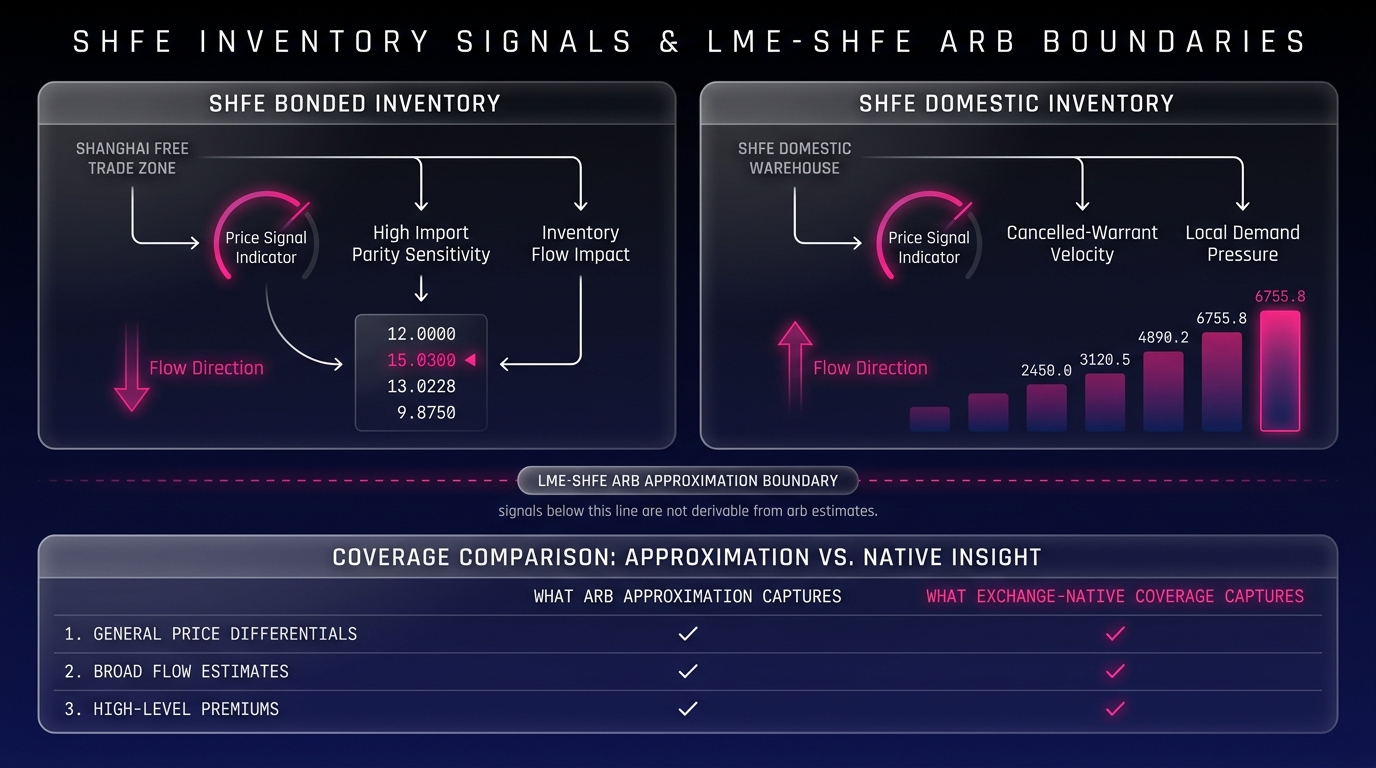
The SHFE warehouse warrant system generates independent price signals that LME-SHFE arbitrage approximations structurally cannot capture. The specific mechanism is cancelled warrant velocity, the rate at which SHFE warehouse warrants are cancelled ahead of physical delivery. To read these signals correctly, traders must distinguish between two structurally separate inventory channels: bonded warehouses and domestic-delivery warehouses. These are not interchangeable signals.
Most metals traders tracking China exposure run the LME-SHFE arbitrage spread as a proxy for Chinese market tightness. That approach does more than underperform in precision. It omits a category of information that exists only inside the SHFE system. According to Shanghai Futures Exchange weekly inventory reports, copper stocks on SHFE have recorded single-quarter fluctuations exceeding 150,000 metric tons, movements that arb-spread approximations registered only after price had already moved.
Understanding how the warrant system works, why bonded and domestic channels are separate price signal environments, and what cancelled warrant velocity reveals gives copper traders an edge that no LME-derived spread can provide.
How the SHFE Warehouse Warrant System Works
The SHFE warehouse warrant system is the mechanism by which physical metal stored in exchange-approved warehouses is represented as a tradeable, transferable instrument. A warrant is issued for each lot of metal that meets SHFE quality and brand specifications upon deposit into a registered warehouse.
Warrants are not inventory counts. They are legal instruments representing ownership of specific physical metal. This distinction matters because warrant status, not total inventory, determines what metal is actually available for delivery against a futures contract.
What is a warehouse warrant in SHFE trading?
A warehouse warrant in SHFE trading is a certificate of title for a specific lot of metal stored in an SHFE-registered warehouse, eligible for delivery against an open futures contract. When a warrant is active, the metal is on-warrant and counts as available exchange inventory. When a holder cancels the warrant, the metal enters the physical withdrawal pipeline and is no longer deliverable on-exchange.
The lifecycle runs in four stages: metal deposited → warrant issued → warrant active (on-warrant) → warrant cancelled → metal physically withdrawn. Each stage carries distinct price implications. The cancellation stage generates the earliest demand signal. Metal does not disappear from inventory statistics until after the cancellation has already telegraphed the intent.
SHFE currently maintains registered warehouse networks across multiple provinces, with copper warrant facilities concentrated in Jiangsu, Guangdong, and Shanghai. According to SHFE data published in 2023, the exchange operates across more than 500 approved warehouse locations in its metals complex, making warrant flow data a genuinely national demand indicator rather than a regional proxy.
Bonded vs. Domestic Inventory: Two Separate Price Channels
This is where non-exchange-native analysis commonly falls short. SHFE copper inventory exists in two structurally distinct environments: bonded warehouses and domestic-delivery warehouses. They are not interchangeable, and aggregating them into a single inventory figure is a consequential analytical error in cross-exchange metals coverage.
Bonded warehouses hold metal that has not yet cleared Chinese customs. This metal is physically located in China but has not entered the domestic economy. It has not paid import VAT (currently 13% for copper cathode) or applicable customs duties. It can be re-exported without triggering domestic tax obligations.
Domestic-delivery warehouses hold metal that has cleared customs and is fully inside the Chinese domestic economy. It has paid all applicable taxes and duties. It can be delivered directly against SHFE futures contracts. Re-export is economically prohibitive under normal market conditions.
How does bonded inventory differ from domestic SHFE inventory?
Bonded inventory differs from domestic SHFE inventory in three fundamental ways: tax status, delivery eligibility, and export optionality. Bonded metal cannot be delivered against SHFE futures contracts. It must first clear customs, pay VAT and duties, and be registered in an SHFE-approved domestic warehouse. Domestic inventory is immediately deliverable on-exchange.
The price implications are therefore structurally different. A spike in bonded inventory signals that arbitrage traders are importing metal speculatively, waiting for the domestic premium to justify clearing costs. A drawdown in domestic inventory with accelerating cancelled warrants signals active physical demand pulling metal out of the exchange system now.
According to Shanghai Metals Market (SMM) research, the premium for VAT-cleared domestic copper over bonded copper in Shanghai has historically ranged between $60 and $200 per metric ton depending on import economics and domestic demand intensity. That spread is itself a price signal, but only if a trader is tracking both channels as separate data series.
Why does aggregate inventory data mislead copper traders?
Aggregate inventory data misleads copper traders because it collapses two channels with opposing price implications into a single number. Rising total inventory could mean bonded stocks are building while domestic on-warrant stocks are simultaneously declining. A trader reading only the aggregate sees flat or rising inventory and misses the domestic tightening signal entirely.
This scenario is not an edge case. During periods of elevated LME-SHFE arbitrage, bonded inventory commonly builds as importers front-load while domestic SHFE warrants cancel at an accelerating pace. The two channels move in opposite directions for structural reasons. According to Metals Focus data, this divergence pattern occurred across three distinct demand cycles between 2020 and 2023, each time generating a domestic spot premium that aggregate inventory figures predicted too late to be actionable.
SHFE copper inventory data methodology bonded versus domestic
Cancelled Warrant Velocity: The Signal That Precedes the Move
Cancelled warrant velocity is the rate of warrant cancellation over a defined time window, typically expressed as the percentage of total on-warrant stocks cancelled within a single weekly SHFE inventory report. It is not equivalent to an inventory drawdown. It precedes one.
Inventory falls after warrants are cancelled and metal is physically withdrawn from exchange warehouses. Cancelled warrant velocity leads the inventory decline by three to ten business days depending on warehouse location and logistics complexity. That lead time is the signal window.
What does cancelled warrant velocity indicate in metals markets?
Cancelled warrant velocity indicates the pace of physical offtake from SHFE-registered warehouses, functioning as a leading indicator of domestic demand intensity. High velocity (cancellations exceeding 10% to 15% of total on-warrant stocks in a single weekly report) typically precedes inventory depletion and cash-to-futures basis strengthening in the domestic market. Low velocity with stable or rising on-warrant stocks signals reduced physical urgency.
The mechanism is direct: a copper fabricator or end-user who needs physical metal for near-term production cancels warrants to initiate withdrawal. Rather than a financial positioning decision, it is a supply-chain commitment with logistics cost and delivery timeline implications. Aggregated across multiple fabricators operating simultaneously in the same window, these cancellation decisions become a measurable demand signal that precedes futures price adjustment.
According to CRU Group analysis, SHFE copper cancelled warrant spikes have historically preceded domestic spot premium strengthening by an average of five to seven trading days. That window represents actionable lead time for a trader with exchange-native data access and a position framework built to use it.
A further precision point: cancellation concentration by warehouse location qualifies the signal. Cancellations concentrated in Jiangsu warehouses, located within the densest copper fabrication corridor in China, indicate specific end-user demand. Broad cancellations distributed across multiple provinces indicate more generalized demand. The velocity number may be identical; the demand character is not.
copper physical demand leading indicators China SHFE
Why LME-SHFE Arbitrage Approximations Miss SHFE Warrant System Signals
The LME-SHFE arbitrage calculation estimates the economic incentive to import copper into China by comparing LME prices (adjusted for freight, insurance, VAT, and import duty) against SHFE domestic futures prices. When the spread is positive, importing is theoretically profitable. When negative, the domestic market is oversupplied relative to import economics.
While useful as a macro indicator, it cannot substitute for SHFE-native signal reading. Treating them as equivalent creates a structural blind spot rather than a mere estimation error. The distinction matters because a structural blind spot cannot be corrected by refining the arb calculation. The omitted information is categorically absent from the model.
Why does the LME-SHFE arbitrage calculation miss SHFE price signals?
The LME-SHFE arbitrage calculation misses SHFE price signals because it measures import economics, not domestic delivery dynamics. The arb spread answers whether bringing new metal into China is profitable today. It says nothing about what is happening to metal already inside the domestic exchange delivery system. Cancelled warrant velocity, domestic basis behavior, and warehouse-level concentration patterns are entirely invisible to arb-based analysis.
The structural omission operates across three separate channels:
- Tax and regulatory timing asymmetry: The arb calculation applies static VAT and duty assumptions. Actual clearing economics vary with regulatory environment, trader-specific import license conditions, and bonded storage carrying costs. Metal sitting in bonded storage because clearing economics are marginal at current spreads represents latent supply, not active supply. The arb spread misrepresents it as immediately available inventory.
- Geographic basis blindness: SHFE registers warehouses across multiple provinces, and regional logistics costs create basis differentials between, for example, copper warranted in Guangdong versus Jiangsu. The LME-SHFE arb is a single national number. It cannot capture the regional tightness that concentrated warrant cancellation patterns in specific provinces reveal.
- Physical pipeline lag: The arb spread reflects current futures pricing. It does not reflect the physical delivery pipeline state. Cancelled warrant velocity captures that pipeline state. It tells you what metal has already committed to leaving the exchange system before the commitment appears in any price feed.
LME-SHFE copper arbitrage spread structural limitations
Reading the SHFE Warehouse Warrant System as a Price Signal
Reading the SHFE warehouse warrant system as a standalone signal generator requires tracking four variables simultaneously: total on-warrant stocks, cancelled warrant volume as a percentage of on-warrant inventory, the bonded-to-domestic stock ratio, and warehouse-level geographic concentration of cancellations. No single variable is sufficient. The signal emerges from their interaction.
A practical analytical workflow for copper:
- Establish the seasonal baseline: What is the normal SHFE copper warrant level for the current calendar month? Chinese New Year and Golden Week generate predictable inventory builds that must be normalized out before velocity signals carry meaning. A 9% cancellation rate in late January reads differently than the same rate in March.
- Track the cancellation rate, not the inventory total: Cancellations above 8% of on-warrant stocks in a single weekly report warrant elevated attention. Above 12%, the signal is active: domestic demand is pulling metal from the exchange system at an above-normal pace that will appear in inventory figures within the following week.
- Cross-check the bonded-to-domestic ratio direction: If bonded stocks are building while domestic warrants cancel at pace, the market is tightening at the domestic level even as total visible inventory appears flat or rising. This is the divergence that aggregate-inventory analysis is structurally blind to.
- Identify warehouse concentration: Broad cancellations distributed across multiple provinces indicate generalized demand pressure. Cancellations concentrated in Jiangsu or Guangdong fabrication hubs indicate specific, production-driven offtake, which tends to sustain longer and convert more reliably into basis strengthening than financially motivated positioning.
China copper demand ICSG global share data
What Exchange-Native SHFE Coverage Means for Position Management
Understanding the SHFE warrant mechanism at this level of granularity redefines what exchange-native coverage means operationally. Beyond simply receiving SHFE price feeds alongside LME quotes, this requires the capacity to interpret warrant flow data within its correct structural context: the bonded and domestic channels as separate signal environments, cancelled warrant velocity as a leading indicator, and arb-spread analysis as a complementary second layer rather than a primary signal.
For a front-office copper trader managing exposure across LME and SHFE, the position management implications are direct and consequential.
A position built on LME technical signals alone is blind to domestic Chinese tightening until it surfaces in LME price action, typically after the move has already begun. A position informed by SHFE cancelled warrant velocity can be structured ahead of that tightening, with the physical signal providing directional conviction before the arb spread confirms it and well before LME spot reflects the full premium compression.
The integrated workflow looks like this: SHFE warrant data on a weekly report cadence feeds a domestic tightness composite alongside bonded inventory direction. That composite generates a signal state (neutral, elevated, or active) that informs position sizing and hedge ratio decisions for copper across exchanges. The LME-SHFE arb spread functions as a second-layer timing tool for supply-flow anticipation, not the primary demand signal.
Legacy CTRM platforms were not designed with this workflow in mind. Most aggregate SHFE inventory into a single line item alongside LME and COMEX stocks, treating all exchange inventory as equivalent for position risk purposes. According to industry analysis cited by Commodity Technology Advisory (ComTech), more than 60% of mid-market metals trading firms report using analytics platforms that do not distinguish bonded from domestic inventory in their risk layer. That architecture makes the bonded-versus-domestic distinction analytically invisible and cancelled warrant velocity unmeasurable. This occurs not because the underlying SHFE data does not exist, but because the platform design has eliminated the channel through which it would be read.
Depth-first SHFE coverage means the warrant mechanism is not an optional feature configured on request. It is the foundation from which SHFE analysis is built. Bonded and domestic channels are labeled separately from the ground up. Cancelled warrant velocity is tracked as a first-class signal with its own indicator logic, not estimated from inventory deltas after metal has already left the system. The arb spread is contextualized within the physical pipeline picture, not used as a substitute for it.
CTRM platform SHFE integration bonded domestic inventory
Conclusion: Build the Signal Layer Before You Build the Position
The SHFE warehouse warrant system generates price signals through a specific, observable mechanism (cancelled warrant velocity operating across two structurally distinct inventory channels) that LME-SHFE arbitrage approximations are structurally unable to replicate. Bonded and domestic inventory are not the same number. The arb spread is not a proxy for domestic tightness. Cancelled warrant velocity leads price by five to ten trading days, which means it is useful only if you are tracking it before you need it.
Three actions to implement immediately:
- Separate bonded and domestic SHFE inventory in every system and data feed. If your platform aggregates them, that is a structural gap requiring correction at the platform architecture level, not a limitation to route around with a spreadsheet.
- Track cancelled warrant percentage weekly as your primary domestic demand signal, not inventory totals as a lagging confirmation. The cancellation rate is the demand pipeline. The inventory total is what remains after the pipeline has already drained.
- Reposition the LME-SHFE arb spread as a supply-flow timing tool, not a tightness indicator. It answers whether metal wants to enter China. Cancelled warrant velocity answers what metal is already exiting the domestic exchange system. Both belong in a complete copper position framework. They answer fundamentally different questions and should be read in sequence, not treated as substitutes.